Code
# install.packages("osmdata",dependencies = TRUE)In this section, I will describe how to build maps for several cities around the world, using global open access mapping data from “osmdata” pacakge in R.
https://docs.ropensci.org/osmdata/articles/osmdata.html.
From the package website, they explain how working with open access map data, ensures transparent data provenance and ownership, allowing anyone to contribute, encouraging democratic decision making and citizen science. OSM is a global open access mapping project, which is free and open under the ODbL licence (OpenStreetMap contributors 2017)
OpenStreetMap (OSM) project information can be accessed via overpass queries using osmdata package in R. This package obtains OSM data from the overpass API, which is a read-only API that serves up custom selected parts of the the OSM map data.
To start working with Open OpenStreetMap package, I first install it from CRAN
# install.packages("osmdata",dependencies = TRUE)And then load it the usual way using pacman::p_load() function to load several libraries at once, pacman::p_load(here,tidyverse,osmdata,sf,showtext). This is a more efficient way of working with several R libraries.
These are the specific From osmdata package we will use these functions to plot our map:
Once I know which features to include in the map (buildings,roads,rivers,lagoons and bays), then I select the relevant tags that constitute the query we pass to the API to plot them using ggplot2. These are the set of osmdata functions used in this section:
These three functions combined provides me with a gggplot2() object I can turn into a map using geom_sf() to handle shape files and polygons.
In a nutshell, a sf object is a collection of simple features that includes attributes and geometries in the form of a data frame. It is a data frame (or tibble) with rows of features, columns of attributes, and a special geometry column that contains the spatial aspects of the features.
For a further explanation about sf objects, please refer to Jesse Sadler website: [sf objects]https://www.jessesadler.com/post/simple-feature-objects/#:~:text=At%20its%20most%20basic%2C%20an,spatial%20aspects%20of%20the%20features.
Then I load some extra libraries for data wrangling and to create plots
pacman::p_load(here,tidyverse,osmdata,sf,showtext)The echo: false option disables the printing of code (only output is displayed).
When building maps using OpenStreetMap, we can think about them in similar terms as ggplot2 plots, in the sense we build them step by step, adding one layer at a time to display the required information on top of the initial map of the region we want to create a map from.
Having selected the city we want to plot, then we use getbb() function to obtain a bounding box for a given place name. In this instance I will plot the city of Valencia in Spain.
getbb() provides latitude and longitude coordinates associated with Valencia city in Spain
getbb("Valencia Spain") min max
x -0.4325512 -0.2725205
y 39.2784496 39.5666089When creating a map of Valencia, it’s important to decide which features to include. In OpenStreetMap, each feature is identified by a key, which is then further subdivided into values.
To plot roads or highways on the map, we first need to identify how these features are defined in the osmdata package. We can do this by using the available_features() function to select different types of roads or transportation routes defined in the map.
Once we have chosen the desired features, we can add them to our map along with other layers to create a comprehensive and informative representation of Valencia.
# Not run as there are more than 250 elements
# available_features()
Looking at the list of available features, I can see that “highway” is one of the keys that I can use to plot transportation routes on my map of Valencia. However, I need to determine which specific values are associated with this key.
To do this, I can use the available_tags() function to identify the values that are related to the “highway” key. By selecting the appropriate values for the key, I can customize the map to display the types of transportation routes that are most relevant to my needs.”
available_tags("highway") [1] "bridleway" "bus_guideway" "bus_stop"
[4] "busway" "construction" "corridor"
[7] "crossing" "cycleway" "elevator"
[10] "emergency_access_point" "emergency_bay" "escape"
[13] "footway" "give_way" "living_street"
[16] "milestone" "mini_roundabout" "motorway"
[19] "motorway_junction" "motorway_link" "passing_place"
[22] "path" "pedestrian" "platform"
[25] "primary" "primary_link" "proposed"
[28] "raceway" "residential" "rest_area"
[31] "road" "secondary" "secondary_link"
[34] "service" "services" "speed_camera"
[37] "steps" "stop" "street_lamp"
[40] "tertiary" "tertiary_link" "toll_gantry"
[43] "track" "traffic_mirror" "traffic_signals"
[46] "trailhead" "trunk" "trunk_link"
[49] "turning_circle" "turning_loop" "unclassified"
[52] "via_ferrata" I plan to begin by mapping the primary roads in Valencia. To do this, I will select a few key tags from the list, such as motorway, primary, secondary, tertiary,residential,living_street, unclassified.
Roads and highways are the first set of elements to be included on my map of Valencia. Displaying transportation routes in the city but also through its metropolitan area. From the previous available_tags() function, I choose “highway” as the appropriate value for this key.
This allows me to display different types of transportation types such as motorways, primary, secondary, and tertiary roads as well as motorways on the map.
# MAP LAYER 01: roads
roads <- getbb("Valencia Spain") %>%
         opq(timeout =  3500) %>%
         add_osm_feature(key = "highway",
                        value = c("motorway","primary","secondary","tertiary",
                                  "residential","living_street","unclassified")) %>%
         osmdata_sf()
roadsIn r, I use the sf cartographic object I obtained from our OpenMap API query, mapping several sf objects via ggplot2 and geom_sf() functions.
Also, using getbb(“Valencia Spain”) function, I ensure the features we display on the map macth the city latitude and longitude I want to plot.
So far I have created just one geom_sf() object, embedded insite the ggplot() function, alongside the lat and long values for the city of Valencia.
Prior to producing the final map, I define the colour palette for each new feature,
# Remember to enclose Hexadecimal colors in apostrophes
road_color <- '#000000'
coastline_color <- '#000000'
Then I can combine all previous scripts to create the first output map:
Valencia_roads_map <- ggplot() +
                  geom_sf(data = roads$osm_lines,
                          inherit.aes = FALSE,
                          color = road_color
                            ) +
                  # Define city coordinates for maps. Given by getbb("Valencia Spain") function
                  coord_sf(xlim = c(-0.4325512, -0.2725205),
                           ylim = c(39.2784496, 39.5666089),
                           expand = FALSE)
Valencia_roads_map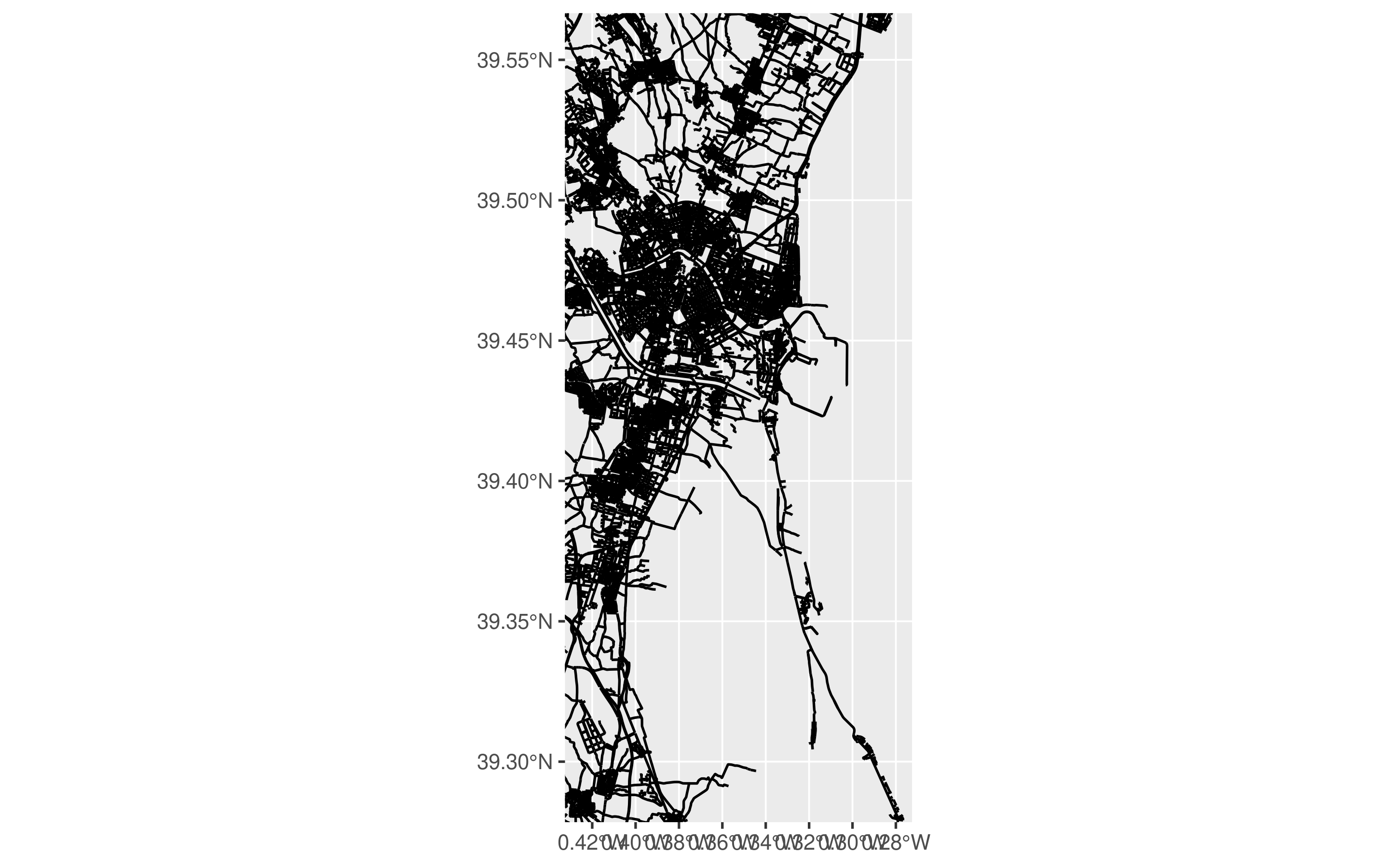
Now I have added a new layer to the previous map, including beaches, dunes, bays and coastline natural water features.
available_tags("natural") [1] "arch" "arete" "bare_rock" "bay"
[5] "beach" "blowhole" "cape" "cave_entrance"
[9] "cliff" "coastline" "crevasse" "dune"
[13] "earth_bank" "fell" "fumarole" "geyser"
[17] "glacier" "grassland" "heath" "hill"
[21] "hot_spring" "isthmus" "moor" "mud"
[25] "peak" "peninsula" "reef" "ridge"
[29] "rock" "saddle" "sand" "scree"
[33] "scrub" "shingle" "shoal" "shrubbery"
[37] "sinkhole" "spring" "stone" "strait"
[41] "tree" "tree_row" "tundra" "valley"
[45] "volcano" "water" "wetland" "wood" These are the set of elements I will include in the map enclosed in the concatenate c() function below: “bay”,“water”,“beach”,“wetland”,“dune”, “coastline” all these are coastline and water related map features.
Vlc_coastline <- getbb("Valencia Spain") %>%
  opq(timeout =  3500) %>%
  add_osm_feature(key = "natural",
                  value = c("bay","water","beach","wetland","dune","coastline")) %>%
  osmdata_sf()
Vlc_coastlineVlc_coastline_multipolygons <- Vlc_coastline$osm_multipolygonsRoads features are defined as lines whilst coastline and water features are defined as multipolygons
MAP 02: Map combining roads and coastline layers
Set colour palette for road and coastline features
road_color <- '#1E212B'
coastline_color <- '#D4B483'# This is the ggplot2() MAP02
Valencia_coastline_map <- ggplot() +
# roads
geom_sf(data = roads$osm_lines,
inherit.aes = FALSE,
color = road_color
) +
# coastline as multipolygons
geom_sf(data = Vlc_coastline_multipolygons,
inherit.aes = FALSE,
color = coastline_color
) +
# Define city coordinates for maps. Given by getbb("Valencia Spain") function
coord_sf(xlim = c(-0.4325512, -0.2725205),
ylim = c(39.2784496, 39.5666089),
expand = FALSE)
Valencia_coastline_map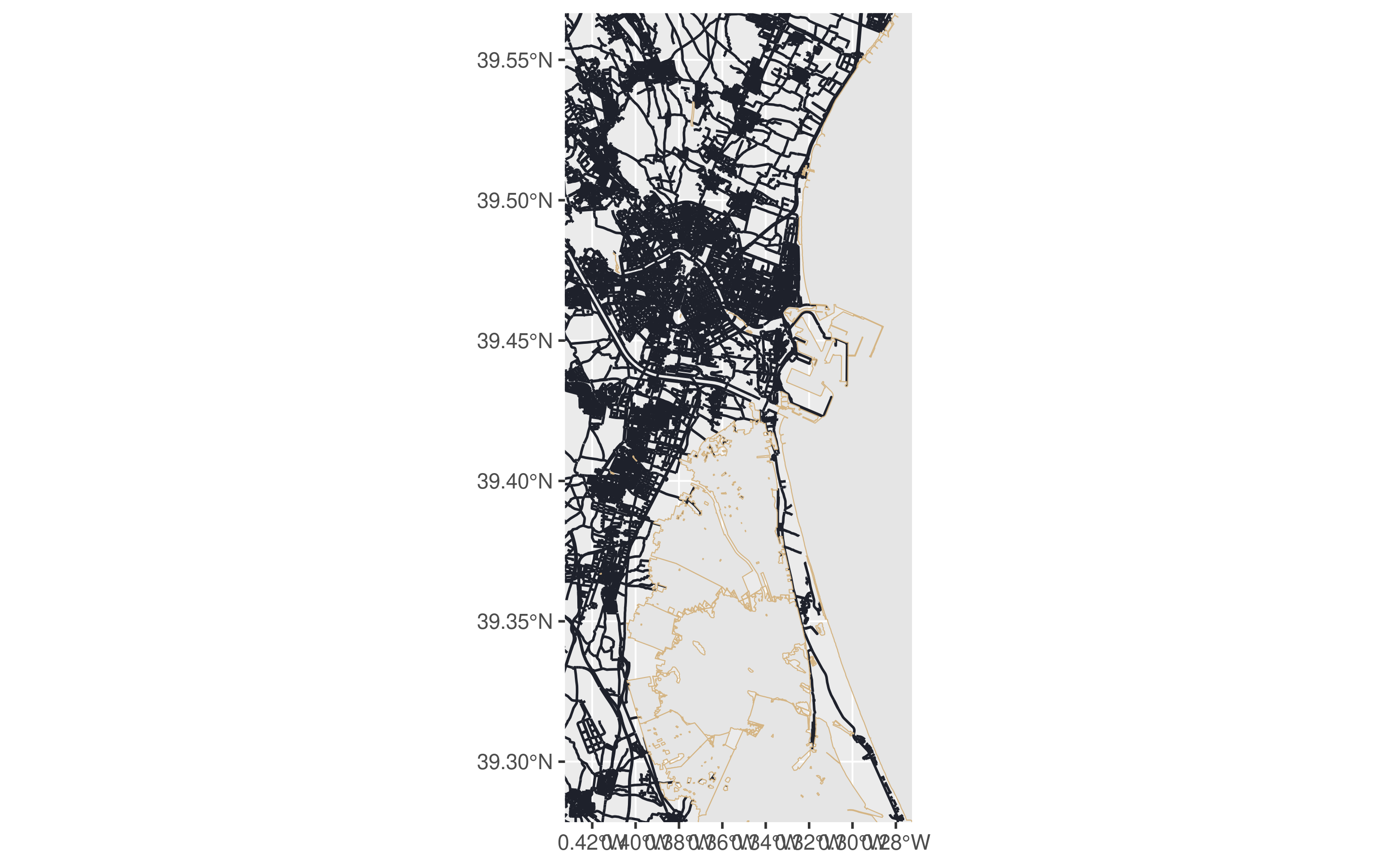
Vlc_water <- getbb("Valencia Spain") %>%
  opq(timeout =  3500) %>%
  add_osm_feature(key = "water") %>%
  osmdata_sf()

Vlc_sea <- getbb("Valencia Spain") %>%
  opq(timeout =  3500) %>%
  add_osm_feature(key = "waterway",
                  value = "river") %>%
osmdata_sf()Vlc_water_multipolygons <- Vlc_water$osm_multipolygons
Vlc_sea_multipolygons <- Vlc_sea$osm_multipolygons# Set colour palette for water features
road_color <- '#1E212B'
coastline_color <- '#D4B483'
water_color <- '#0066CC'
waterway_color <- '#99CCFF'# This is the ggplot2() MAP03
Valencia_waterways_map <- ggplot() +
# roads
geom_sf(data = roads$osm_lines,
inherit.aes = FALSE,
color = road_color
) +
# coastline as multipolygons
geom_sf(data = Vlc_coastline_multipolygons,
inherit.aes = FALSE,
color = coastline_color
) +
# water colour as multipolygons
geom_sf(data = Vlc_water_multipolygons,
inherit.aes = FALSE,
color = water_color
) +
# waterway colour as multipolygons
geom_sf(data = Vlc_sea_multipolygons,
inherit.aes = FALSE,
color = waterway_color
) +
# Define city coordinates for maps. Given by getbb("Valencia Spain") function
coord_sf(xlim = c(-0.4325512, -0.2725205),
ylim = c(39.2784496, 39.5666089),
expand = FALSE)
Valencia_waterways_map 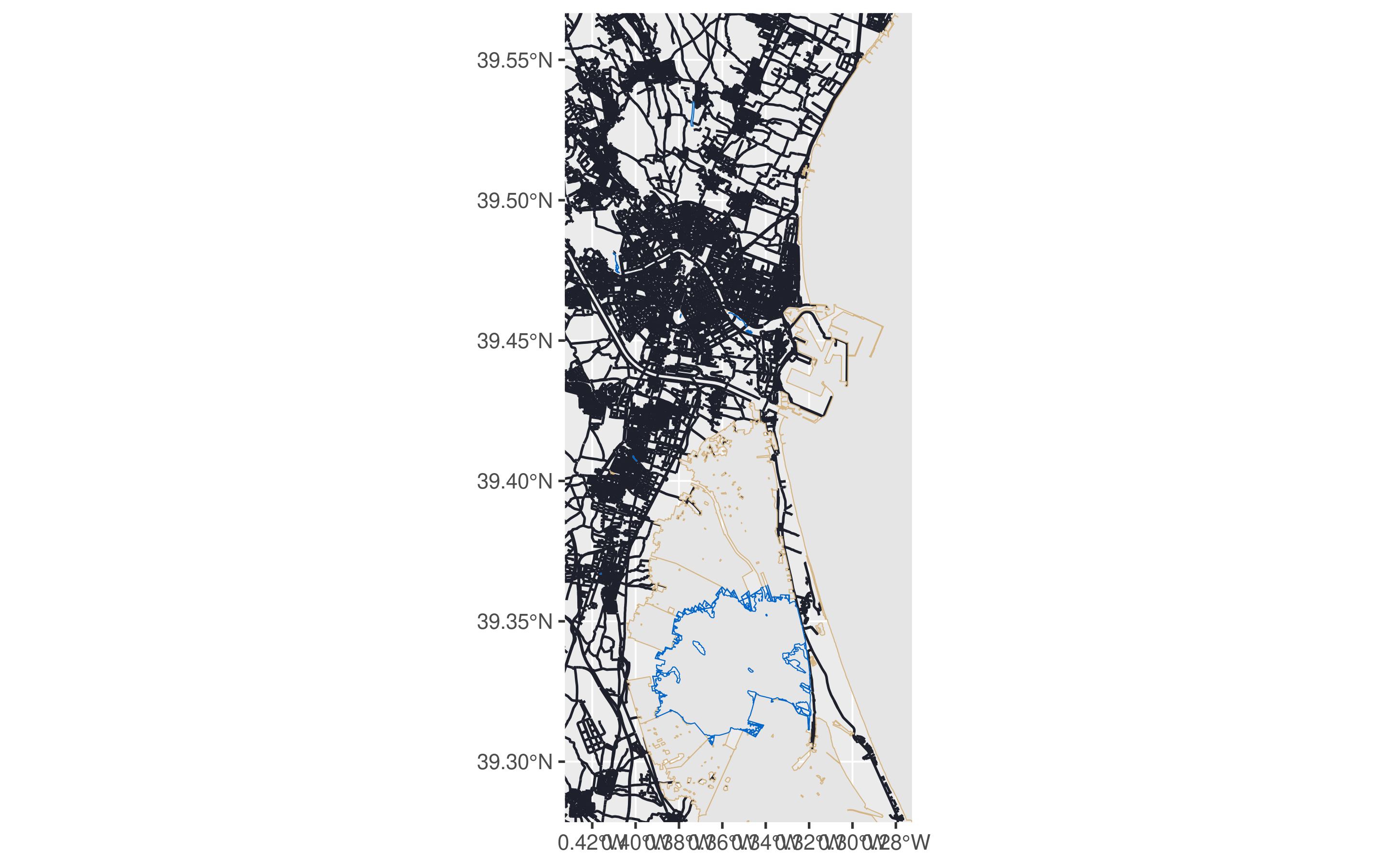
After defining several features to be plotted in the map (roads,coastline,waterways and rivers), I combine them as ggplot2 plot layers. To finally create one single ggplot2 image output as a .png file.
This final step also includes enhancing the map appearance by applying several theme options, adding background colour and Title and Subtitle to the output map.
road_color <- '#1E212B'
coastline_color <- '#D4B483'
water_color <- '#0066CC'
waterway_color <- '#99CCFF'
albufera_lagoon <- "#0ACDFF"
font_color <-'#D2691E'
background_color <- "#D4B483"
Themed and formatted final output map of Valencia city
Valencia_city_map <- ggplot() +
  # roads
  geom_sf(data = roads$osm_lines,inherit.aes = FALSE,color = road_color) +
  # coastline
  geom_sf(data = Vlc_coastline_multipolygons,inherit.aes = FALSE, fill = waterway_color, color = waterway_color) +
  # water colour as multipolygons
  geom_sf(data = Vlc_water_multipolygons,inherit.aes = FALSE, fill = water_color, color = water_color) +
  # waterway colour as multipolygons
  geom_sf(data = Vlc_sea_multipolygons,inherit.aes = FALSE, fill = waterway_color, color = waterway_color) +
  # Define city coordinates for maps. Given by getbb("Valencia Spain") function
  coord_sf(xlim = c(-0.4325512, -0.2725205),ylim = c(39.2784496, 39.5666089),expand = FALSE) +
  # Include Map title and subtitle
  labs(title = "Valencia ~ l'Albufera", subtitle = '39.4699° N, 0.3763° W') +
  # Apply specific theme to map title and sub-title
  theme_void() +
  theme(
    plot.title = element_text(family = "Barlow",color = font_color,size = 9,
                              hjust = 0, vjust = 1),
    plot.title.position = "plot",
    plot.subtitle = element_text(family = "Barlow",
                                 color = font_color,
                                 size = 5,
                                 hjust = 0 , vjust = 2.3),
    # Setup background color for entire map
    panel.border = element_rect(colour = background_color, fill = NA, size = 1),
    panel.margin = unit(c(0.6,1.6,1,1.6),"cm"),
    plot.background = element_rect(fill = background_color)
  )

Valencia_city_map 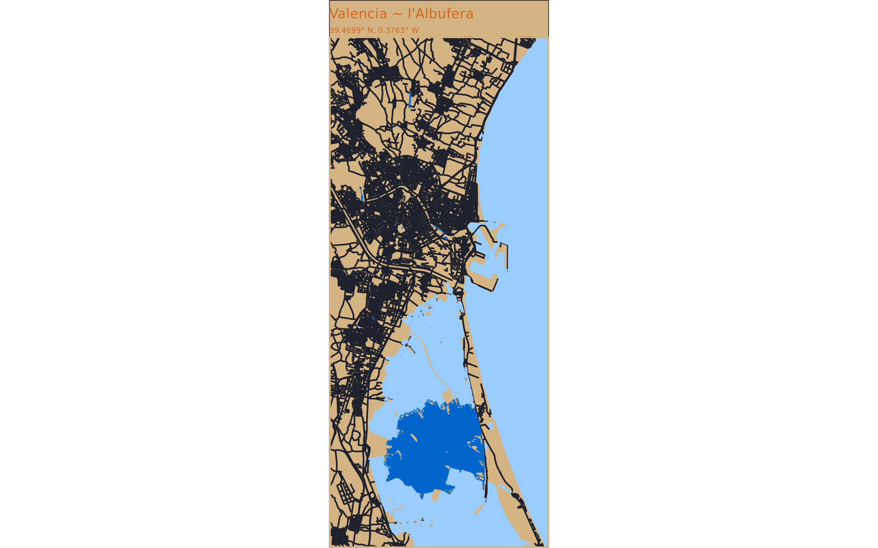
The default image width and height values can be changed to match a standard frame to hang it on the wall as a city map poster.
name <- "Valencia_open_street_map"
width = 20
height = 40
The last step is to use ggsave() function to create an output .png file that to be exported and printed.
ggsave(here::here(paste(name,".png", sep ="_")),
       device = "png", width = width, height = height, units = "cm", dpi = "retina", bg = "transparent")
In coming weeks new city maps of The Hague, Netherlands and Birmingham, UK will be added to this section.
Valencia city map output image as .png file https://github.com/Pablo-source/Maps-in-R/blob/main/City_maps/Valencia_open_street_map_.png
Valencia city map R script https://github.com/Pablo-source/Maps-in-R/blob/main/City_maps/Valencia_open_street_map.R
Similar quarto document to the one used to build this website https://github.com/Pablo-source/Maps-in-R/blob/main/Documentation/Quarto_markdown%20custom%20setup.qmd